
The rate at which the running time increases as a function of Input is called rate of growth:-
| Time Complexity (Big O) | Name | Description (Easy Explanation) |
|---|---|---|
| O(1) | Constant Time | The program takes the same amount of time no matter how large the input is. ⚡ Example: Accessing an element in an array. |
| O(log n) | Logarithmic Time | Time increases slowly even when input grows fast. 📉 Example: Binary Search. |
| O(n) | Linear Time | Time grows directly with the size of the input. 📈 Example: Traversing a list. |
| O(n log n) | Line Logarithmic Time | Slightly more than linear but better than quadratic. ⚙️ Example: Merge Sort, Quick Sort (average case). |
| O(n²) | Quadratic Time | Time grows as the square of the input size. 🧮 Example: Nested loops like in Bubble Sort. |
| O(n³) | Cubic Time | Time grows as the cube of input size — very slow. 🐢 Example: 3 nested loops. |
| O(2ⁿ) | Exponential Time | Time doubles with every extra input element — extremely slow. 🚫 Example: Solving recursive problems like the Traveling Salesman brute-force method. |
| O(n!) | Factorial Time | The worst of all — grows faster than exponential! 😵 Example: Generating all permutations of n elements. |
How to remember this :-
O(1) → Best
O(log n) → Great
O(n) → Good
O(n log n) → Acceptable
O(n²) → Slow
O(2ⁿ), O(n!) → Avoid
What is Time Complexity?
When we analyze an algorithm, we want to know how efficiently it performs.
The Time Complexity tells us how much time an algorithm takes to run as a function of the size of the input (n).
Because performance can vary depending on input, we consider three cases:
1-> Best Case(Omega Notation)
2-> Worst Case(O-Big O Notation)
3-> Average Case(Theta Notation)
1. Best Case (Omega Notation)
Definition:
The best case is the scenario in which the algorithm performs the minimum number of steps or takes the least possible time.
Defines the input for which the algorithm takes the least time (Fastest time to complete).
Input is the one for which the algorithm runs faster.
One may require less memory space other may require less cpu time to execute.
When it occurs:
It happens when the input data is most favorable for the algorithm.
Example:
In Linear Search,
if the element you are searching for is at the first position,
the algorithm stops immediately — that’s the best case.
Representation:
Ω(f(n)) — Omega Notation represents the best-case time complexity.
Example Table:
| Algorithm | Best Case | Example Condition |
|---|---|---|
| Linear Search | O(1) | Element found at the first position |
| Binary Search | O(1) | Element found at the middle in the first comparison |
| Bubble Sort | O(n) | Array already sorted |
2. Worst Case (O – Big O Notation)
Definition:
Defines the input for which the algorithm takes along time.
Input is the one for which the algorithm runs the slowest.
The worst case is the scenario where the algorithm takes the maximum possible time to complete.
When it occurs:
It happens when the input data is least favorable or requires maximum steps.
Example:
In Linear Search,
if the element is not present or at the last position,
the algorithm checks every element — that’s the worst case.
Representation:
O(f(n)) — Big O Notation represents the worst-case time complexity.
Example Table:
| Algorithm | Worst Case | Example Condition |
|---|---|---|
| Linear Search | O(n) | Element not found or at last |
| Binary Search | O(log n) | Element not found after multiple divisions |
| Bubble Sort | O(n²) | Array sorted in reverse order |
3. Average Case (Θ – Theta Notation)
Definition:
Provides a prediction about the running time of the algorithm.
The average case is the expected time an algorithm takes for all possible inputs, assuming that each input is equally likely.
Run the algorithm many times,using many different inputs that come from some distribution that generates these inputs compute the total running time (by adding their individual times) and divides by the number of trials.
When it occurs:
It represents the typical running time of an algorithm under normal conditions.
Example:
In Linear Search,
if the element could be anywhere, on average, the algorithm will check n/2 elements.
Representation:
Θ(f(n)) — Theta Notation represents the average-case time complexity.
Example Table:
| Algorithm | Average Case | Example Condition |
|---|---|---|
| Linear Search | O(n/2) → O(n) | Element present randomly |
| Binary Search | O(log n) | Element found after some divisions |
| Quick Sort | O(n log n) | Randomly ordered input |
5. Comparison Summary:
| Case Type | Meaning | Time Representation | Example (Linear Search) |
|---|---|---|---|
| Best Case | Fastest possible execution | Ω(f(n)) | Found at 1st position |
| Average Case | Expected / normal performance | Θ(f(n)) | Found in middle |
| Worst Case | Slowest possible execution | O(f(n)) | Not found |
6. Real-Life Analogy
Imagine you’re looking for your key in a drawer of 10 items:
| Case | Description |
|---|---|
| Best Case | You find the key in the first try. |
| Average Case | You find it after checking around half of the items. |
| Worst Case | The key is at the last item, or not in the drawer at all. |
7. Why It Matters
- Best case helps you know the minimum possible time.
- Worst case helps in guaranteeing performance (especially for critical systems).
- Average case reflects real-world behavior.
8. Amortize Running Time:
Amortize running time refer to the time required to perform a sequence of related operations averaged over all the operations performed.
Amortized analysis guarantees the average performance of each operations in the worst case.
9. Expressing Time and Space Complexity:
Time and Space complexity can be expressed using a function f(n) where n is the INPUT SIZE for a given instance of the problem being solved.
Expressing the compexity is required when :-
We want to predict the rate of growth of compexity as the input size of the problem increase.
There are multiple algorithms that find a solution to given problem and we need to find the algorithm that is most efficient .
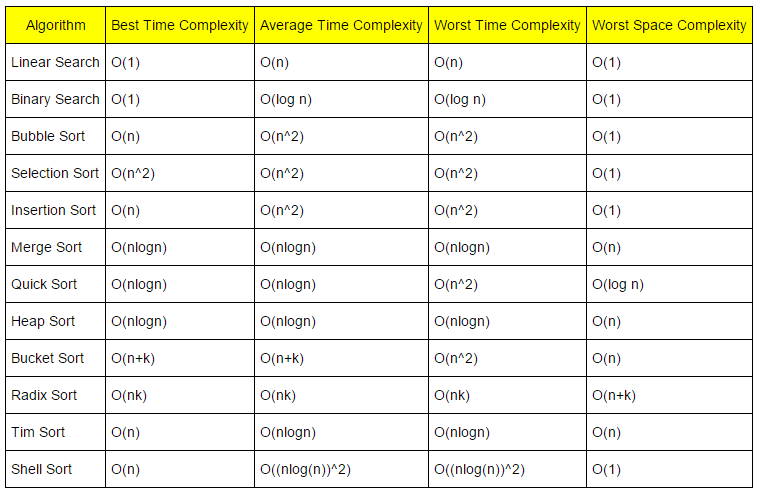
10. All Algorithms Time and Space Complexity(cheatsheet):
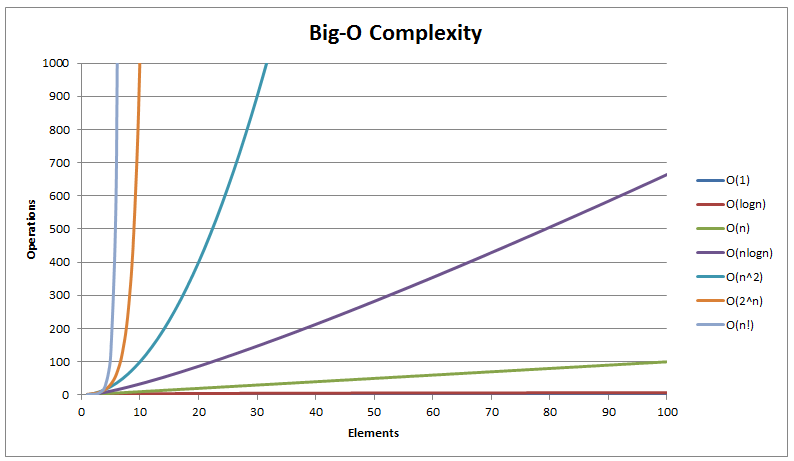
11: Big-O graph:-
Data Structure Operations Cheat Sheet:
| Data Structure | Time Complexity (Average) | Time Complexity (Average) | Time Complexity (Average) | Time Complexity (Average) | Time Complexity (Worst) | Time Complexity (Worst) | Time Complexity (Worst) | Time Complexity (Worst) | Space Complexity (Worst) |
|---|---|---|---|---|---|---|---|---|---|
| Access | Search | Insertion | Deletion | Access | Search | Insertion | Deletion | ||
| Array | Θ(1) | Θ(n) | Θ(n) | Θ(n) | O(1) | O(n) | O(n) | O(n) | O(n) |
| Stack | Θ(n) | Θ(n) | Θ(1) | Θ(1) | O(n) | O(n) | O(1) | O(1) | O(n) |
| Queue | Θ(n) | Θ(n) | Θ(1) | Θ(1) | O(n) | O(n) | O(1) | O(1) | O(n) |
| Singly Linked List | Θ(n) | Θ(n) | Θ(1) | Θ(1) | O(n) | O(n) | O(1) | O(1) | O(n) |
| Doubly Linked List | Θ(n) | Θ(n) | Θ(1) | Θ(1) | O(n) | O(n) | O(1) | O(1) | O(n) |
| Skip List | Θ(log n) | Θ(log n) | Θ(log n) | Θ(log n) | O(n) | O(log n) | O(log n) | O(log n) | O(n log n) |
| Hash Table | N/A | Θ(1) | Θ(1) | Θ(1) | N/A | O(n) | O(n) | O(n) | O(n) |
| Binary Search Tree | Θ(log n) | Θ(log n) | Θ(log n) | Θ(log n) | O(n) | O(n) | O(n) | O(n) | O(n) |
| Cartesian Tree | N/A | Θ(log n) | Θ(log n) | Θ(log n) | N/A | O(n) | O(n) | O(n) | O(n) |
| B-Tree | Θ(log n) | Θ(log n) | Θ(log n) | Θ(log n) | O(log n) | O(log n) | O(log n) | O(log n) | O(n) |
| Red-Black Tree | Θ(log n) | Θ(log n) | Θ(log n) | Θ(log n) | O(log n) | O(log n) | O(log n) | O(log n) | O(n) |
| Splay Tree | N/A | Θ(log n) | Θ(log n) | Θ(log n) | N/A | O(n) | O(n) | O(n) | O(n) |
| AVL Tree | Θ(log n) | Θ(log n) | Θ(log n) | Θ(log n) | O(log n) | O(log n) | O(log n) | O(log n) | O(n) |
| KD Tree | Θ(log n) | Θ(log n) | Θ(log n) | Θ(log n) | O(n) | O(n) | O(n) | O(n) | O(n) |
For Best case operations,the time complexities O(1).