Asymptotic notations :

1. It serves as the foundation of algorithm analysis, categorized into two three type of analysis.
2. These notations are mathematical tool used to analyze the performance of algorithms by understanding how their efficiency changes as the input size grows.
3. These notations provide a concise way to express the behavior of an algorithm’s time or space complexity as the input size approaches infinity.
4. Rather than comparing algorithm directly, asymptotic analysis focuses on understanding the relative growth rates of algorithms complexities.
5. According to the input size increases these notations are used to analyze the performance or time and space complexity

There are many asymptotic notations:

1)Big-O Notation (O-notations) (worst case time complexity)

2)Big-O (Upper Bound)

3)Omega Notation(Ω-notations) (Best case time complexity)

4)Big Omega (Lower Bound)

5)Theta Notation(Θ-notations) (average case time complexity)

6)Big Theta (Tight Bound)

7)Small-O (Strictly Less Than)

8)Small-Omega (Strictly Greater Than)

But mainly there are three notations :-

1. Big-O Notation (O-notations) (worst case time complexity)
2. Omega Notation(Ω-notations) (Best case time complexity)
3. Theta Notation(Θ-notations) (average case time complexity)

1)Big-O notations: –

1. Big-O shows the upper limit of an algorithm’s running time.
2. ·  It tells us the slowest possible growth rate.
3. ·  It’s used to measure worst-case performance.
4. ·  Written as O(f(n)), where f(n) is a function of input size n.
5. ·  It helps in comparing two algorithms easily.
6. ·  Big-O ignores small terms and constants.
7. ·  Example: O(n²) grows faster than O(n).
8. ·  If an algorithm is O(n²), it means time increases quadratically with n.
9. ·  O(1) → Constant time (fastest).
10. ·  O(log n) → Logarithmic time (e.g., Binary Search).
11. ·  O(n) → Linear time (e.g., Linear Search).
12. ·  O(n log n) → Linearithmic time (e.g., Merge Sort).
13. ·  O(n²) → Quadratic time (e.g., Bubble Sort).
14. ·  O(2ⁿ) → Exponential time (e.g., Recursive Fibonacci).
15. ·  Big-O helps predict performance for large inputs.
16. ·  It defines the upper bound—the algorithm will not exceed it.
17. ·  It’s often shown in worst-case analysis tables.
18. ·  It’s one of the most important notations in computer science.
19. ·  It ensures developers avoid inefficient algorithms.
20. ·  Example summary: If a code is O(n), it means doubling n doubles the time.

2)Big-O (Upper Bound) — Detailed View

1. Big-O represents the maximum possible time an algorithm can take.
2. It’s the ceiling of performance growth.
3. The algorithm never exceeds this growth rate.
4. It’s used to guarantee performance limits.
5. Example: O(n²) → At most proportional to n².
6. Even if sometimes it’s faster, it won’t be slower than O(n²).
7. It’s a safe estimate for the worst performance.
8. It is used in algorithm analysis and proofs.
9. The function f(n) defines the upper curve of growth.
10. For small n, constants may matter; for large n, they don’t.
11. Big-O helps compare scalability of algorithms.
12. It’s usually shown in performance charts and graphs.
13. Example: In sorting algorithms, Bubble Sort = O(n²).
14. Merge Sort = O(n log n), so it’s faster for big inputs.
15. It shows how time increases as input size grows.
16. The Big-O curve is always above or equal to actual time.
17. It’s useful when predicting worst performance in systems.
18. It does not depend on hardware—only logic.
19. It is the most commonly used asymptotic notation.
20. In simple words: Big-O = “The algorithm takes at most this much time.”

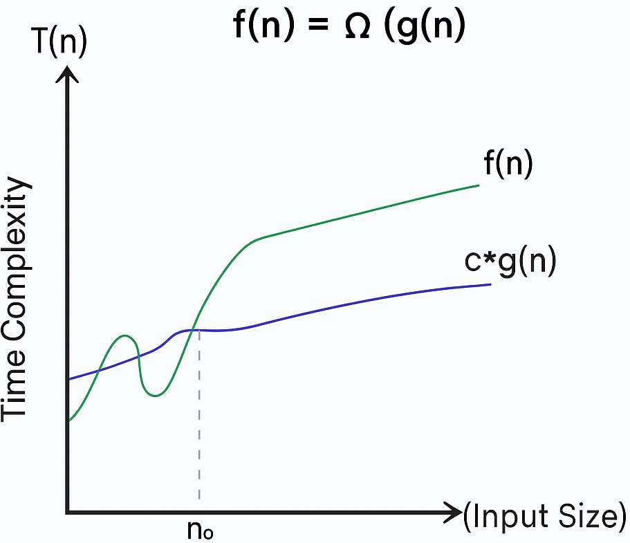
3)Omega Notation (Ω-Notation) — Best Case Time Complexity.

4)Big-Omega(Lower Bound) — Detailed Explanation.

1. In short: Big Omega = “Algorithm will take no less than this much time.”
2. Big Omega defines the lowest boundary of an algorithm’s growth.
3. It’s the best possible case for time complexity.
4. The algorithm won’t perform better than this bound.
5. Example: Ω(n) → Time will be at least linear.
6. It helps in knowing the minimum effort required.
7. It’s useful when comparing best performance limits.
8. In sorting algorithms: Bubble Sort → Ω(n), Merge Sort → Ω(n log n).
9. It means Merge Sort will take at least n log n even in best cases.
10. It represents the lower edge of the complexity graph.
11. The curve of Ω lies below or touches the actual performance.
12. It ensures algorithm designers know the baseline speed.
13. It’s important for benchmark analysis.
14. Ω is used in asymptotic analysis just like Big-O.
15. The real running time of any algorithm lies between Ω and O.
16. If both Ω and O are the same → algorithm has a tight bound.
17. It shows the minimum limit of time complexity.
18. It’s often combined with Θ (Theta) for balanced view.
19. Omega gives a positive side of algorithm performance.
20. It’s written as T(n) ≥ c * f(n) for large n (where c is constant).

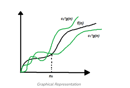
5)Theta Notation (Θ-Notation) -Average Case Time Complexity.

1. In short: Θ = “Algorithm usually takes this much time.
2. Theta (Θ) notation shows the average-case performance of an algorithm.
3. It gives a tight bound on time complexity — both lower and upper limits.
4. It means the algorithm will take approximately this much time in most cases.
5. It’s written as Θ(f(n)), where f(n) is a function of input size.
6. Example: If an algorithm takes Θ(n²), it means it grows roughly proportional to n².
7. Θ is a combination of Big O and Big Omega.
8. In other words, Θ = between the best and worst case.
9. Formula: c₁·f(n) ≤ T(n) ≤ c₂·f(n) for some constants c₁, c₂.
10. It represents balanced performance analysis.
11. Θ(n) → linear average performance.
12. Θ(log n) → logarithmic average performance.
13. Θ(n log n) → efficient algorithms like Merge Sort.
14. Used to show expected behavior of algorithm in normal conditions.
15. If an algorithm’s best, worst, and average cases are same → use Θ.
16. Example: Binary Search = Θ(log n).
17. Example: Bubble Sort = Θ(n²) average case.
18. It’s very useful in practical performance prediction.
19. Θ helps developers know what happens most of the time.
20. It’s the most realistic measure for normal input conditions.

6)Big Theta (Tight Bound) – Balanced Growth Rate

1. Big Theta shows the tight bound of algorithm’s growth.
2. It defines both upper and lower limits accurately.
3. It tells that the algorithm’s performance is neither faster nor slower than f(n).
4. Example: Θ(n²) means it grows exactly like n².
5. The function f(n) is sandwiched between two constants (lower & upper).
6. It’s written mathematically as:
   → ∃ constants c₁, c₂ > 0, and n₀ > 0, such that
   c₁·f(n) ≤ T(n) ≤ c₂·f(n) for all n > n₀.
7. It gives the most accurate complexity of an algorithm.
8. If Big O = Big Omega = Θ → algorithm has a perfect bound.
9. It helps to describe exact rate of growth.
10. Example: Merge Sort = Θ(n log n).
11. Binary Search = Θ(log n).
12. Linear Search = Θ(n).
13. Bubble Sort = Θ(n²).
14. It is the most preferred notation in asymptotic analysis.
15. It shows that algorithm grows proportionally with input size.
16. It’s used when performance variation is minimal.
17. It represents stable and predictable algorithms.
18. Θ notations help in runtime estimation accurately.
19. It means the growth rate will always stay near f(n).
20. In short: Big Theta = “Algorithm grows exactly at this rate.”

7)Small-o notation is written as o(f(n)).

1. It represents an upper bound that is not tight.
2. It means the algorithm grows slower than f(n).
3. Example: If T(n) = o(n²), it means T(n) grows slower than n².
4. Small-o excludes equality — only strictly less than.
5. It’s like saying: “T(n) grows less quickly than f(n).”
6. Used when the algorithm is more efficient than f(n).
7. Formally: For every constant c > 0, there exists n₀ such that
8. T(n) < c·f(n) for all n > n₀.
9. It’s a loose upper limit — not exact.
10. Big-O allows equality, but small-o does not.
11. Example: log n = o(n)
12. Example: n = o(n²)
13. Example: n² ≠ o(n²) (because it’s equal, not strictly less)
14. Used in mathematical proofs of algorithm growth.
15. It indicates better performance than some function.
16. It’s rarely used in basic algorithm analysis — mostly theoretical.
17. o(f(n)) means “eventually smaller than f(n)” as n → ∞.
18. It helps to express tighter comparisons between growth rates.
19. It’s useful when analyzing limit-based performance.
20. In short: Small-o = “grows slower than f(n), but not equal.”

In short: Small-o = “grows slower than f(n), but not equal.”

8)Small-Omega Notation (Strictly Greater Than – Lower Bound That’s Not Tight)

1. In short: Small-omega = “grows faster than f(n), but not equal.”
2. Small-omega notation is written as ω(f(n)).
3. It represents a lower bound that is not tight.
4. It means the algorithm grows faster than f(n).
5. Example: T(n) = ω(n) means T(n) grows faster than n.
6. It’s the opposite of small-o.
7. It excludes equality — only strictly greater than.
8. Used when the algorithm is less efficient than f(n).
9. Formally: For every constant c > 0, there exists n₀ such that
10. T(n) > c·f(n) for all n > n₀.
11. It’s a loose lower limit — not exact.
12. Big-Omega allows equality, but small-omega does not.
13. Example: n² = ω(n) ✅
14. Example: n log n = ω(n) ✅
15. Example: n² ≠ ω(n²) ❌ (equal is not allowed)
16. It shows that T(n) grows significantly faster than f(n).
17. Used in theoretical comparisons of algorithms.
18. Helps identify algorithms that are slower than a given rate.
19. ω(f(n)) means “eventually greater than f(n)” as n → ∞.
20. It’s often used in asymptotic proofs in complexity theory.
21. Example: n² = ω(n log n).

Notation	Symbol	Meaning	Relation Type	Example
Big-O	O(f(n))	Upper Bound	≤ or =	T(n) ≤ c·f(n)
Omega	Ω(f(n))	Lower Bound	≥ or =	T(n) ≥ c·f(n)
Theta	Θ(f(n))	Tight Bound	=	c₁·f(n) ≤ T(n) ≤ c₂·f(n)
Small-o	o(f(n))	Strictly Less	<	log n = o(n)
Small-omega	ω(f(n))	Strictly Greater	>	n² = ω(n)

Summary of Growth Notations:-

Notation	Symbol	Meaning	Represents	Use Case	Mathematical Form	Example
Big-O	O(f(n))	Upper Bound	Worst Case	To show the maximum growth rate	T(n) ≤ c·f(n), ∀ n ≥ n₀	T(n) = 2n² + 3n + 1 → O(n²)
Big-Omega	Ω(f(n))	Lower Bound	Best Case	To show the minimum growth rate	T(n) ≥ c·f(n), ∀ n ≥ n₀	T(n) = 2n² + 3n + 1 → Ω(n²)
Big-Theta	Θ(f(n))	Tight Bound	Average Case	When both upper and lower bounds are same	c₁·f(n) ≤ T(n) ≤ c₂·f(n)	T(n) = 2n² + 3n + 1 → Θ(n²)
Small-o	o(f(n))	Strictly Less	Loosely Faster	When T(n) grows slower than f(n)	∀ c > 0, ∃ n₀ s.t. T(n) < c·f(n)	log n = o(n)
Small-Omega	ω(f(n))	Strictly Greater	Loosely Slower	When T(n) grows faster than f(n)	∀ c > 0, ∃ n₀ s.t. T(n) > c·f(n)	n² = ω(n)

For Visual Understanding (in Words):-

Imagine a ladder of growth from slowest to fastest

O(1)  →  O(log n)  →  O(n)  →  O(n log n)  →  O(n²)  →  O(n³)  →  O(2ⁿ)  →  O(n!)

Now —

• Big-O (O): says “T(n) grows no faster than this level.”
• Big-Omega (Ω): says “T(n) grows no slower than this level.”
• Big-Theta (Θ): says “T(n) grows exactly at this level.”
• Small-o (o): says “T(n) grows strictly slower than this level.”
• Small-Omega (ω): says “T(n) grows strictly faster than this level.”

Real-World Example

Let’s take a car race :-

Concept	Meaning in Race
Big-O (O)	The maximum speed limit the car can reach.
Big-Omega (Ω)	The minimum speed the car maintains.
Big-Theta (Θ)	The average consistent speed of the car.
Small-o (o)	A car that’s slower than another, but never matches it.
Small-Omega (ω)	A car that’s faster than another, but never equal.

FOR recap:-

1. Learning these helps you optimize your code and predict scalability.
2. Asymptotic notations help compare algorithm efficiency.
3. Big-O focuses on upper limit / worst case.
4. Omega (Ω) focuses on lower limit / best case.
5. Theta (Θ) gives exact growth (tight bound).
6. Small-o means strictly smaller growth.
7. Small-Omega (ω) means strictly larger growth.
8. Together, they form a complete asymptotic analysis toolkit.
9. These notations are used to ignore constants and lower-order terms.
10. They help compare algorithms independent of hardware or environment.